Lab 2B - Tangent Planes
Math 2374 - University of Minnesota
http://www.math.umn.edu/math2374
questions to: rogness@math.umn.edu, drake@math.umn.edu
Introduction
In last week's lab, we investigated properties of continuity, differentiability, and partial derivatives. In this lab, all of the functions we consider will be differentiable, which as we learned means that we can approximate the function at any given point with a linear approximation, or "tangent plane."
There's an important point here: earlier we talked about whether a function is differentiable at the point ![Overscript[x, ⇀] = Overscript[a, ⇀]](HTMLFiles/index_1.gif) ; if we say that a function is "differentiable" without any modifier, we mean that it is differentiable at every point, or at least every point where it is defined. Go to the following web page:
; if we say that a function is "differentiable" without any modifier, we mean that it is differentiable at every point, or at least every point where it is defined. Go to the following web page:
http://www.math.umn.edu/~rogness/multivar/tanplane.shtml
(Or, alternatively, expand the subsection below labeled "Tangent Plane Example" and evaluate the cell there.) This demo shows you part of a paraboloid with a tangent plane at a certain point; you can click and drag the point to move it around, and LiveGraphics3D will automatically show you the tangent plane at the new point.
This is intended to reinforce the point that a "differentiable" function doesn't have one single tangent plane (or linear approximation, if you prefer that language). Rather, it has a different linear approximation at each point!
Today we'll learn various methods of finding the equation of the tangent plane / linear approximation of a differentiable function. In some sense this is one of the most important things you can learn in this course, and all of the material for the first month of the class has led to this point. You'll even get a foreshadowing of things to come; in lecture, you've learned what the gradient is, but you haven't learned all of its properties. In this lab you'll see how you can use the gradient to find a tangent plane, which will be mentioned later in the book an in lecture.
Tangent Plane Example
Plotting Planes
Before we begin considering issues of tangency, let's review how to plot planes. It might help you to look in your textbook and review Cartesian and parametric equations for planes; you can also ask your TA for help.
The nicest situation is when we can describe the plane as a function of x and y; in that case, we can write the equation of the plane as ``z = ax + by + c'' where a, b, and c are real numbers. We can just use Plot3D in those cases; for instance, if we had z = 3x - y, we could just use
In[92]:=
![Plot3D[3x - y, {x, -2, 2}, {y, -2, 2}]](HTMLFiles/index_3.gif)
![[Graphics:HTMLFiles/index_4.gif]](HTMLFiles/index_4.gif)
Out[92]=
to plot the plane, adjusting the range of x and y if necessary.
Even if we can describe a plane with a nice, easy equation, it is sometimes more convenient or enlightening to describe the plane with parametric equations. If we are given a point and two non-parallel vectors, there is a unique plane containing that point parallel to each of the vectors. Let's say our vectors are (2,3,5) and (-7,-11,13), and we wish to find the plane parallel to those two vectors passing through the point (17, 29, 0). In parametric equations, we could write

where s and t range over all real numbers. To plot this plane, we use the properties of scalar multiplication and vector addition, and use ParametricPlot3D:
In[93]:=
![ParametricPlot3D[{17 + 2 * t - 7 * s, 29 + 3 * t - 11 * s, 5 * t + 13 * s}, {t, -1, 1}, {s, -1, 1}]](HTMLFiles/index_7.gif)
![[Graphics:HTMLFiles/index_8.gif]](HTMLFiles/index_8.gif)
Out[93]=

You can keep the parametric equation of the plane in ``un-multiplied out'' form and use ParametricPlot3D, although earlier versions of Mathematica might complain a bit before showing you the graph. Either way works; mathematically they are exactly equivalent. The following form may be easier to write.
In[94]:=
![ParametricPlot3D[{17, 29, 0} + t * {2, 3, 5} + s * {-7, -11, 13}, {t, -1, 1}, {s, -1, 1}]](HTMLFiles/index_10.gif)
![[Graphics:HTMLFiles/index_11.gif]](HTMLFiles/index_11.gif)
Out[94]=

One important thing to note is that we've only plotted a small portion of the plane. Above we chose values of t and s between -1 and 1, but we can choose any range we like. The ranges on s and t don't have to be the same. You don't have to use s and t if you don't like; Mathematica will let you use pretty much any variable name you like. The world is your oyster.
There's one other point you should be aware of. In this class you've seen how difficult it can be sometimes to represent three-dimensional pictures on a two-dimensional computer screen or piece of paper. A picture of a plane can be particularly hard to decipher; it's sometimes difficult to tell which part is sloping uphill, which part is going downhill, or even whether a plane is horizontal or vertical. As an example, look at the previous picture and try to decide how the plane is situated in space. Then evaluate the following command, which will make the same picture pop up in an interactive window. Rotate the plane around and see how accurately you interpreted the two-dimensional picture.
In[95]:=
![ParametricPlot3D[{17, 29, 0} + t * {2, 3, 5} + s * {-7, -11, 13}, {t, -1, 1}, {s, -1, 1}]](HTMLFiles/index_13.gif)
![[Graphics:HTMLFiles/index_14.gif]](HTMLFiles/index_14.gif)
Out[95]=

Example
Plot the plane that's described by
![RowBox[{s (0, 0, 1), , +, , RowBox[{t, RowBox[{(, RowBox[{0.2, ,, , 0.2, ,, , 2}], )}]}]}]](HTMLFiles/index_16.gif)
when s and t range from 2 to 3. It won't look very good—it's ``too skinny''. Experiment with some different ranges on s and t until you get a nicer picture—one that's a little more ``square''.
Exercise 1 - A Thought Experiment
Are there planes that are not the graph of a function of x and y? If so, which planes are they? If there are no such planes, explain why.
Are there planes that cannot be described by a parametrization? If so, which planes are they? If there are no such planes (i.e., any plane whatsoever can be described by a parametrization), explain why.
Explain your reasoning!
Tangent Planes Via Partial Derivatives
You've learned that, basically, a function is "differentiable" if it has a linear approximation; in the case of a function  , this is the same as saying it has a tangent plane at each point. You've also seen the general (cartesian) equation
  of a linear approximation/tangent plane for a function like this; it has lots of partial deriatives in it.
In this section we're going to learn how to use partial derivatives to find the parametric equation of a tangent plane. Before you do anything else, open the following page in a web browser and read the material there:
http://www.math.umn.edu/~rogness/multivar/partialderivs.html
Once you've read the web page, you can continue on to the rest of the lab.
Using Tangent Vectors to find Parametric Equations of Tangent Planes
So now you've seen that tangent vectors of cross sections through a point are in the tangent plane at that point. But wait -- all we need to write down the parametric equation of a plane is a point on the plane and two vectors in the plane! So, in this situation, we've got all the information we need. Given two cross sections of a surface which intersect at a point ![Overscript[x, ⇀] = Overscript[a, ⇀]](HTMLFiles/index_19.gif) , the equation of the tangent plane is:
, the equation of the tangent plane is:
![p(s, t) = Overscript[a, ⇀] + s · (tan . vector of first cross section at the point Overs ... pt[a, ⇀]) + t · (tan . vector of second cross section at the point Overscript[a, ⇀]) .](HTMLFiles/index_20.gif)
Let's do a real-life example now, by finding the plane tangent to the surface
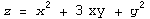
at the point (1,-2,-1). First let's plot the surface; we'll use the Mesh option to turn off the grid, so that later on we can see our cross sections a little better.
In[96]:=
![f[x_, y_] = x^2 + 3 x * y + y^2 surf = Plot3D[f[x, y], {x, 0, 2}, {y, -3, -1}, MeshFalse, AxesLabel {"x", "y", "z"}]](HTMLFiles/index_22.gif)
Out[96]=

![[Graphics:HTMLFiles/index_24.gif]](HTMLFiles/index_24.gif)
Out[97]=

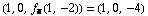
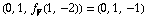
Now we need to find the partial derivatives of f and evaluate them at the point  .
.
In[98]:=
![fx[x_, y_] = D[f[x, y], x] fy[x_, y_] = D[f[x, y], y] fx[1, -2] fy[1, -2]](HTMLFiles/index_27.gif)
Out[98]=

Out[99]=

Out[100]=

Out[101]=

As you learned in the external web page, the vectors
are both parallel to the tangent plane at our point; let's use the Arrow3D graphics object to draw these vectors with our surface. The syntax for Arrow3D might seem a little odd; we have to tell Mathematica that it's a graphical object (hence the Graphics3D[] bit), and then we tell it the starting point and ending point of the vector. Make sure you can understand why the following command does that.
In[102]:=
![tangentvectorx = Graphics3D[Arrow3D[{1, -2, -1}, {1, -2, -1} + {1, 0, -4}]] ; tangentvectory = ... 3D[Arrow3D[{1, -2, -1}, {1, -2, -1} + {0, 1, -1}]] ; Show[surf, tangentvectorx, tangentvectory] ;](HTMLFiles/index_34.gif)
![[Graphics:HTMLFiles/index_35.gif]](HTMLFiles/index_35.gif)
We're using ShowLive here instead of Show because you'll probably have to rotate the picture and look at it from below to see the vectors. It certainly seems plausible that they're in a tangent plane for the surface!
Let's go ahead and define the parametric equation for our tangent plane, using the equation above.
In[105]:=
![p[s_, t_] = {1, -2, f[1, -2]} + s * {1, 0, fx[1, -2]} + t * {0, 1, fy[1, -2]}](HTMLFiles/index_36.gif)
Out[105]=

Now plot the plane and the surface together in a LiveGraphics3D pop-up window:
In[106]:=
![tanplane = ParametricPlot3D[p[s, t], {s, -1, 1}, {t, -1, 1}] ; Show[surf, tanplane] ;](HTMLFiles/index_38.gif)
![[Graphics:HTMLFiles/index_39.gif]](HTMLFiles/index_39.gif)
![[Graphics:HTMLFiles/index_40.gif]](HTMLFiles/index_40.gif)
Rotate the picture and see if you can convince yourself that this plane really is tangent to the surface. (We've talked about how appearances can be deceiving, but in this case your eyes aren't lying to you.) Note how the plane is above the surface at some points and below it at others; that's perfectly fine. It's analogous to the line tangent to the curve y =  at x = 0, which goes above and beneath the curve:
In[108]:=
![Plot[{Sin[x], x}, {x, -Pi/2, Pi/2}, AspectRatioAutomatic]](HTMLFiles/index_42.gif)
![[Graphics:HTMLFiles/index_43.gif]](HTMLFiles/index_43.gif)
Out[108]=

Using Tangent Vectors to find Cartesian Equations of Tangent Planes
Sometimes we need to find a Cartesian equation for a tangent plane. Recall that the Cartesian equation of a plane looks like

where  is a point on the plane, and the vector
  is normal (i.e. perpendicular) to the plane. Now think back to what we've been doing so far: given a surface, we choose a point; then we find two curves through that point; then we find the tangent vectors at that point.
So we've got a point, and now we need a normal vector. Why not just use the cross product of the two tangent vectors? They're both in the tangent plane, so their cross product is perpendicular to the plane.
Here's the parametric equation of the tangent plane we just found, which touches the surface at  .
.
In[109]:=
![p[s_, t_] = {1, -2, f[1, -2]} + s * {1, 0, fx[1, -2]} + t * {0, 1, fy[1, -2]}](HTMLFiles/index_49.gif)
Out[109]=

The two tangent vectors are  and
and  , so our normal vector is their cross product. Mathematica can compute cross products with a command named, not surprisingly, Cross:
In[110]:=
![Cross[{1, 0, -4}, {0, 1, -1}]](HTMLFiles/index_53.gif)
Out[110]=

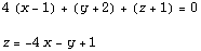
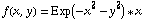
Therefore our Cartesian equation for this same plane is
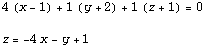
Let's plot this using Plot3D and show it with the original surface:
In[111]:=
![tanplane2 = Plot3D[-4x - y + 1, {x, 0, 2}, {y, -1, -3}] ; Show[surf, tanplane2] ;](HTMLFiles/index_56.gif)
![[Graphics:HTMLFiles/index_57.gif]](HTMLFiles/index_57.gif)
![[Graphics:HTMLFiles/index_58.gif]](HTMLFiles/index_58.gif)
Are you convinced that this is the same tangent plane? It certainly looks that way, and in fact it is!
Exercise 2
In this exercise you're going to find the linear approximation (or tangent plane, if you prefer) of the function  at the point
  . Your work should include the following steps:
(a) Describe the cross sections of the surface defined by  and
and  .
.
(b) Find the partial derivatives of g at the appropriate point; using these values, find two vectors tangent to the surface there.
(c) Give simplified parametric and cartesian equations for the tangent plane.
Your writeup should include a good picture of both the surface and the tangent plane. You should put some thought into the ranges of the x- and y-values in your picture; if you're too close, you won't be able to tell the difference between the plane and the surface, but if you're too far away, the resulting picture may not be very useful. In particular, if your picture clearly shows that your plane is not tangent, or if it's impossible to tell, you will most likely lose points.
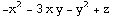
Exercise 3
In this exercise you're going to find the linear approximation (or tangent plane, if you prefer) of the function 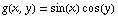 at the point
 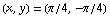 . Your work should include the following steps:
(a) Describe the cross sections of the surface defined by  and
and  .
.
(b) Find the partial derivatives of g at the appropriate point; using these values, find two vectors tangent to the surface there.
(c) Give simplified parametric and cartesian equations for the tangent plane.
Your writeup should include a good picture of both the surface and the tangent plane. You should put some thought into the ranges of the x- and y-values in your picture; if you're too close, you won't be able to tell the difference between the plane and the surface, but if you're too far away, the resulting picture may not be very useful. In particular, if your picture clearly shows that your plane is not tangent, or if it's impossible to tell, you will most likely lose points.
Tangent Planes Via Gradients
Another way to find the tangent plane to a surface is to use the gradient vector. Recall that the gradient vector of a function f(x,y) is defined to be
![Overscript[∇, ⇀] f (x, y) = (∂f/∂x, ∂f/∂y) .](HTMLFiles/index_67.gif)
Hmmm. This is a two-dimensional vector, and to define a plane in 3-space, we'll definitely need vectors with three components. We get around this by doing some minor rearranging. Our surface is defined by  . We could move everything over to the same side and say that our surface is defined by the equation

You might be thinking that this is an odd step; if anything, it's a more complicated way to write it. That's true, and it's going to get a little worse. Rather than saying our surface is defined by this equation, let's defined a new function:

And now we say that our function is the level set defined by  . So now instead of the nice, simple statement
  , we're suddenly talking about level sets. Yikes! There's a reason for this, however...
Notice that  is a function of three variables, and its gradient
![Overscript[∇, ⇀] g (x, y, z) = (-∂f/∂x, -∂f/∂y, 1) .](HTMLFiles/index_75.gif)
Now recall from lecture that the gradient of a function g is perpendicular to the level sets of g. (If you haven't seen this in lecture yet, you will soon. Just take it for granted here; it might be a good idea to ask your TA to draw a picture of what this means.) In other words:
-- We can start with a point (x,y,z) which is on the level set  .
.
-- Because of the way we defined  , this is the same as saying the point is on the surface
  .
.
-- Furthermore, ![Overscript[∇, ⇀] g (x, y, z)](HTMLFiles/index_79.gif) will be perpendicular (or normal) to our surface at that point.
will be perpendicular (or normal) to our surface at that point.
-- In particular, we can use ![Overscript[∇, ⇀] g (x, y, z)](HTMLFiles/index_80.gif) as a normal vector to define the equation for our tangent plane!
as a normal vector to define the equation for our tangent plane!
Let's use this method quickly to find the same tangent plane we've been working with this whole time. Remember that the function is given by:
In[113]:=
![f[x_, y_] = x^2 + 3 x * y + y^2](HTMLFiles/index_81.gif)
Out[113]=

So we can do our magic "new" function like this:
In[114]:=
![g[x_, y_, z_] = z - f[x, y]](HTMLFiles/index_83.gif)
Out[114]=
We're interested in the gradient at the point  :
:
In[115]:=
![gradg[x_, y_, z_] = Grad[g[x, y, z]] gradg[1, -2, -1]](HTMLFiles/index_86.gif)
Out[115]=

Out[116]=

Thus the Cartesian equation of the tangent plane is:
Which is exactly what we found before. Good!
Although the "gradient method" of finding a tangent plane might seem more complicated -- particularly if you don't like level sets -- it's very, very useful. We didn't have to find any cross sections, find tangent vectors, and so on. We just rewrote the original equation, computed one gradient, and we were basically done!
Exercise 4
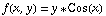
Use the gradient method to find the cartesian equation of the plane tangent to
at the point  Show the graph of f(x,y) and this tangent plane together on the same plot. Be sure to show your work and explain your reasoning.
Exercise 5
Use the gradient method to find the cartesian equation of the plane tangent to
at the point 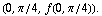 Show the graph of f(x,y) and this tangent plane together on the same plot; use the ranges -π to π for both x and y. Be sure to show your work and explain your reasoning. In particular, with the suggested ranges the "true" tangent plane looks like it sticks through part of the surface. You may want to explain why that's the case.
Tangent Plane Conspiracy Theory
You are not responsible for the material in this section, but we've included it for those people who are interested in the mathematics behind all of this; it turns out that all of the different methods of finding tangent planes aren't really all that different!
In this section, we'll learn that, despite all appearances to the contrary, the ``tangent vectors'' and ``gradient vector'' methods are surreptitiously working together and are engaged in a secret government conspiracy!
Okay, there's no government conspiracy (well...none that I'm aware of), but it is true that the two methods are working together—in fact, they are just different ways of looking at the same thing. Let's talk about directional derivatives for a bit before explaining why they're the same.
Above we were talking about partial derivatives and directions, which should remind you of directional derivatives. In the Tangent Vectors section, when specifying ``the planes y = 2x - 4 and y = -x - 1'', we were really talking about direction vectors. In the above cases, the corresponding direction vectors would be
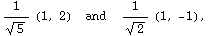
respectively. We are basically using the slope of a line: y = 2x - 4 is a line (in two dimensions) with slope 2. The vector (1,2) is parallel to that line, and above we just normalized it. The other direction vector was obtained in a similar way. Once we know direction vectors, we just need to take the dot product with the gradient vector to find the directional derivative. The conspiracy is already unravelling.
For the function f(x,y) =  at the point (1,-2), and the first direction vector—call it u—we have

We interpret this by saying ``in the direction of u, f is increasing at a rate of  .'' The upshot of this is that (
 ,
,  ,
,  ) is a tangent vector to f(x,y), and it's parallel to (1,2,-6)—the tangent vector we found by using the path we described in the first section. We get this vector by taking the direction vector—a two-dimensional vector—and adding a third component, which is given by the directional derivative of f(x,y). In general, this means that
is a vector tangent to the surface z = f(x,y). You should do this same process with the other direction vector above and make sure that you end up with a tangent vector parallel to (1,-1,-3).
Of course, there's nothing special about those two directional vectors above. We can use any two non-parallel direction vectors and we'll get the same plane—which is exactly what you would hope for, since a function can have only one tangent plane (or no tangent plane, if the function isn't differentiable). The following exercise will help you expose the conspiracy—er, show that the tangent planes from the ``tangent vectors method'' and from the ``gradient vectors method'' are in fact the same. We'll do that by comparing the normal vectors of the resulting planes.
Exercise
(Notice that this isn't in a red box; you don't have to hand this exercise in. You might find it interesting, however.)
As discussed in the Gradient Vector section, the gradient of z - f(x,y) represents a normal vector to the tangent plane, so our main objective is to find the normal vector of the plane we get from the tangent vector method. We'll use an arbitrary differentiable function f(x,y) and two non-parallel direction vectors u = (u1, u2) and v = (v1, v2).
(i) Find the vectors tangent to f(x,y) in the directions of u and v. Describe them in terms of u1, u2, v1, v2, and the partials of f (∂f / ∂x and ∂f / ∂y).
(ii) Find the normal vector of the plane spanned by those two vectors.
(iii) Show that the normal vector you found in (ii) is parallel to the gradient vector of the function g(x,y,z) = z - f(x,y).
(iii) What does this imply about the tangent planes found using the two different methods?
Credits
Created by
Mathematica
(October 4, 2004)